Measuring the Power of Small Engines

Home Model Engine Machinist Forum

Help Support Home Model Engine Machinist Forum:

This site may earn a commission from merchant affiliate links, including eBay, Amazon, and others.

romartin

Well-Known Member
Joined
Jun 4, 2012
Messages
117
Reaction score
66
[SIZE=+2]AN INSTRUMENT FOR MEASURING THE POWER DELIVERED BY SMALL ENGINES[/SIZE]
INTRODUCTION
This thread briefly presents an instrument I have developed during the last year to try to measure the delivered power of the small steam engines I have built over the years. I took the basic idea for the instrument from the chapter Testing Model Engines in K.N. Harris’s classic Model Stationary and Marine Steam Engines. This idea was the object of a patent by a certain Mr. Sellers in the early 1900s.

PRINCIPLE OF OPERATION

As we know power is defined as energy per unit of time, and energy is defined as force multiplied by distance. In the MKS metric system which I use Time is measured in seconds, Distance in meters, Mass in kilograms, Force in newtons (the force needed to accelerate a mass of 1 Kg at the rate of 1 meter/sec/sec); Pressure in pascals (1 newton per square meter), Energy in joules (the energy needed to move 1 meter against a force of 1 newton) and Power in watts (1 joule per second). At the surface of the earth the force of gravity on a mass of 1 Kg is taken to be 9.81 newtons. Since 1 pascal is a very small pressure, I will use the bar as the unit of pressure. 1 bar is equal to 100,000 pascals and is very nearly equal to one atmosphere.
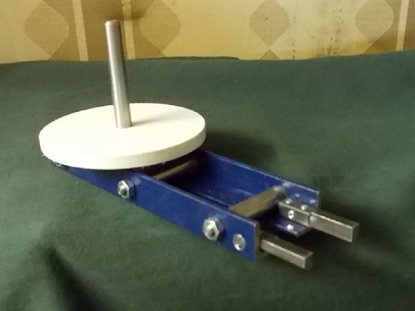
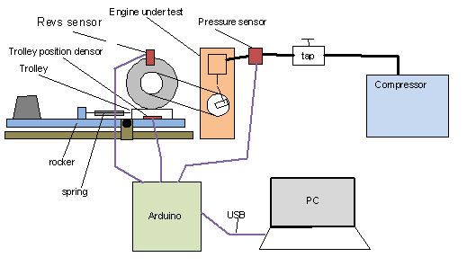
The instrument presented in Harris’s book measures power by direct application of the above definitions. The image below, taken from Harris’s book, illustrates the principle.

P1-01SellersDynamometer_zps7309d22e.jpg


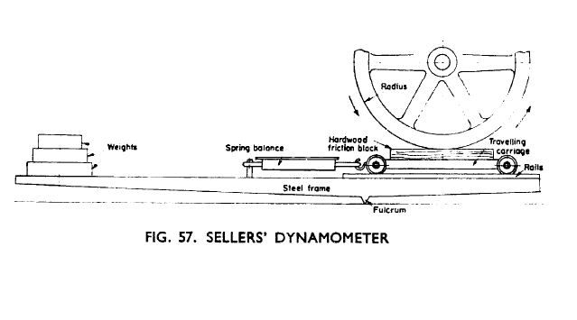
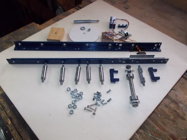
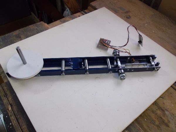
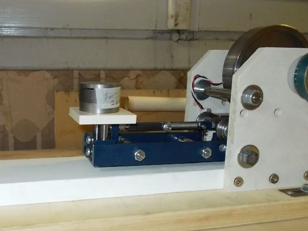
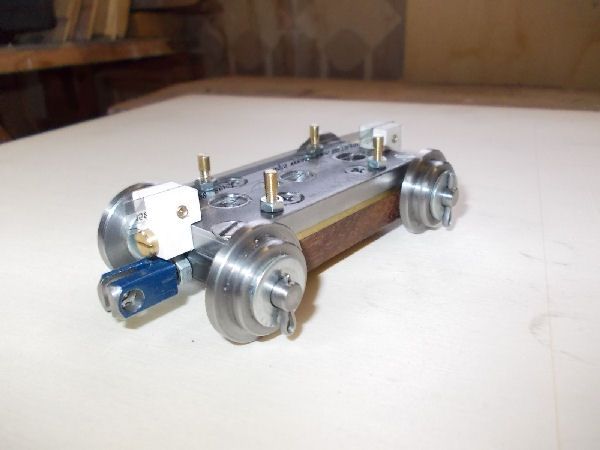
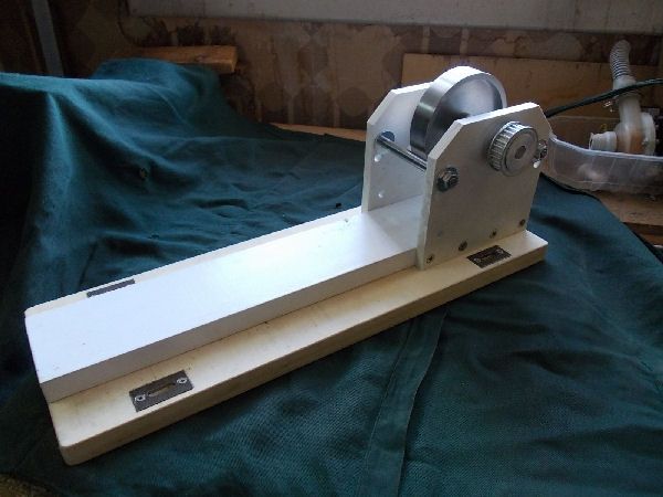
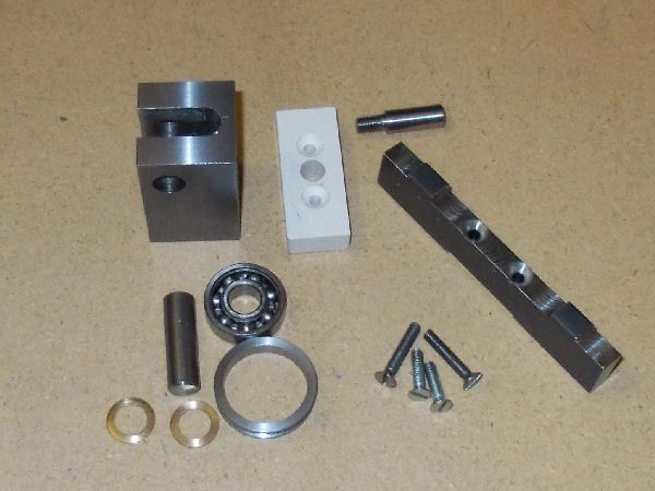
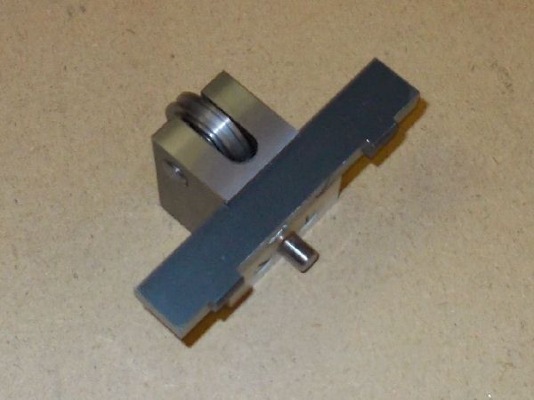
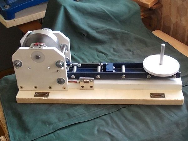
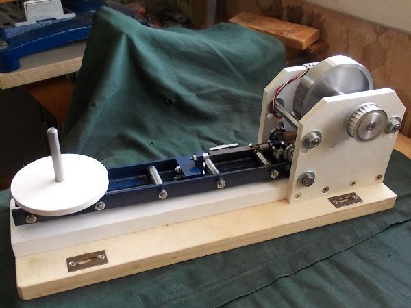
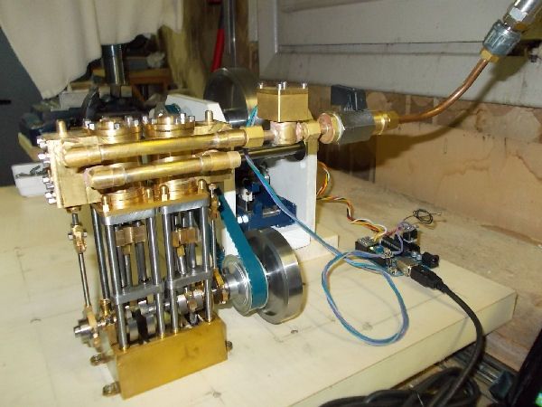
The engine to be measured must drive a brake wheel of the instrument. This wheel is braked by a block of waxed hardwood pressed against its rim. This wooden block is mounted on a trolley which can move along a rail tangent to the wheel rim and which is fixed to the business end of a spring balance. The tangential frictional drag between the wheel and the block is thus directly measured by the spring balance. The rails on which the trolley moves are in turn mounted at one end of a pivoted rocker; on the other end of the rocker is a platform on which weights can be placed to adjust the pressure of the wooden block against the wheel rim.
The spring balance is designed to measure mass by using the earth’s gravitational force on that mass, so its reading of mass in kilograms must be multiplied by 9.81 to obtain the frictional force in newtons. For each revolution of the wheel the distance moved against this force is simply the length of the wheel’s circumference. Thus for each revolution of the wheel the energy in joules developed by the engine under test is this force in newtons multiplied by that length in meters. Multiply this energy in joules by the number of revolutions per second and you have the engine’s delivered power in watts.


Thus to calculate the engine’s power the instrument must measure two things:
  • the tangential frictional force between the wheel and the block,
  • the revolution rate of the wheel.
Clearly the power output by a steam engine depends on the temperature and pressure of the steam. Furthermore only by knowing these values can we estimate the power consumed by the engine and hence estimate the engine’s efficiency. Since at least initially I will be doing the testing using compressed air I can dispense with the temperature measurement but I must have a pressure sensor at the engine’s input. Then an estimate of the power in watts consumed by the engine is given by the input gauge pressure in pascals multiplied by the cylinder cross section in square meters multiplied by the piston stroke length in meters multiplied by the number of power strokes per revolution (4 for a two cylinder double acting engine) multiplied by the engine revolutions per second.
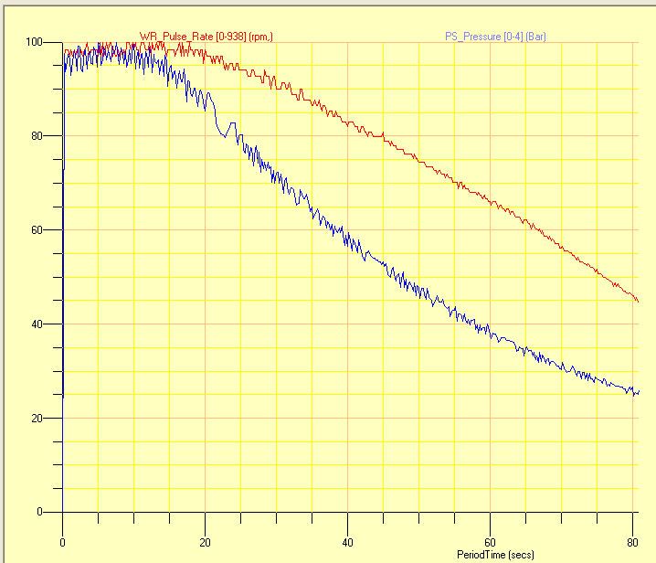
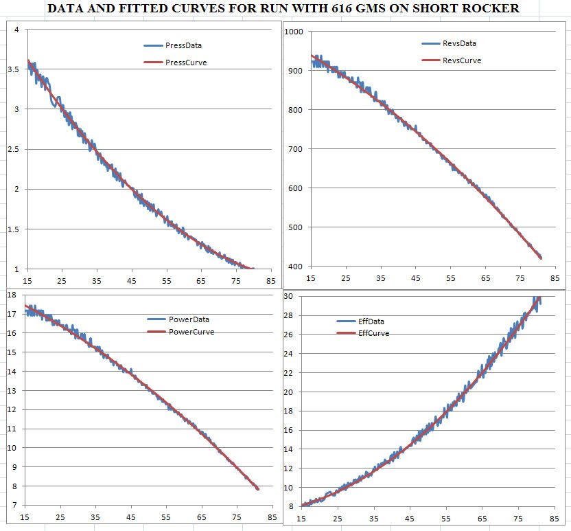
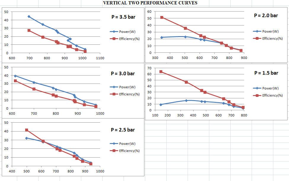
With constant input conditions (pressure, temperature..), one would expect the both the power and the efficiency of a steam engine to be a function of the revs, perhaps presenting a peak at some optimal value of the revs.

ENTER ARDUINO

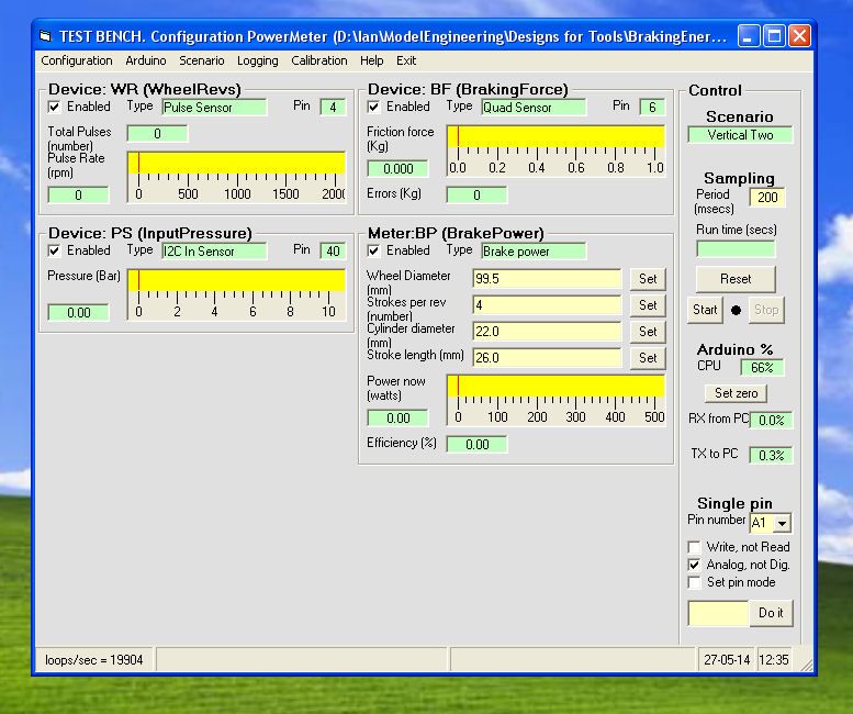
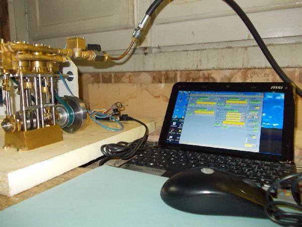
My early attempts to find a means for measuring the revolution rate of a wheel led me to the idea of using an Arduino microprocessor, which actually costs significantly less than a dedicated rev meter and which opens up other fascinating opportunities. So I bought one and took it and my small portable PC with me to play with during my long summer break in the north of Italy away from my workshop. I thoroughly enjoyed this encounter and have become an enthusiastic Arduino fan. The result of my fun is a software tool Test Bench most of which runs on the PC connected via USB to Arduino and which not only measures the revolution rate but can sample and record for subsequent analysis other real time data captured by the Arduino.

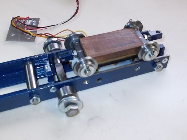
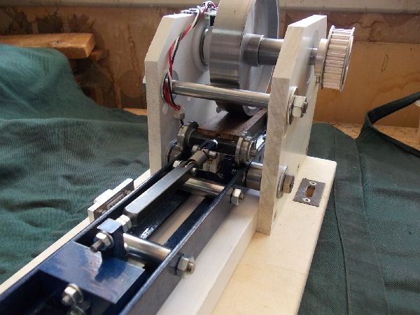
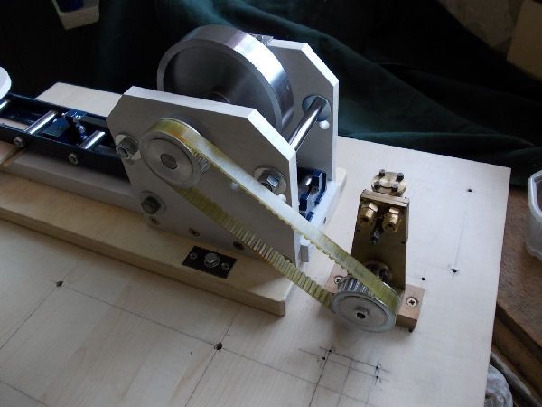
An infrared fork sensor costing a few euro (Photologic Slotted Optical Switch OPB626) is used to provide an Arduino digital input with a square wave at the revolution frequency. The axle of the wheel drives a disc with a suitable cutout to allow the infrared beam to pass for only half of each revolution. Arduino measures the time between successive upward transitions and the PC uses this to give a precise rpm estimate of the instantaneous rev rate. I have tested this solution up to over 3000 rpm.
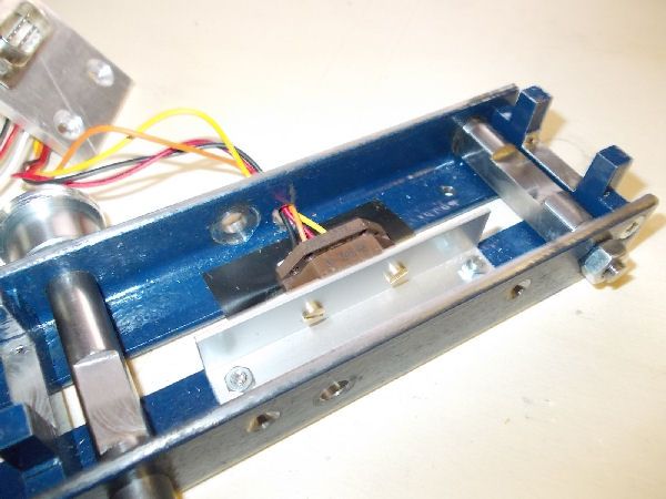
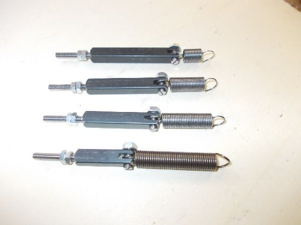
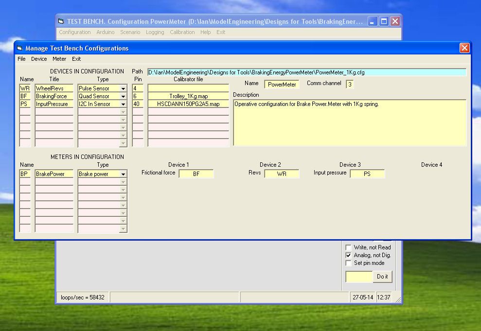
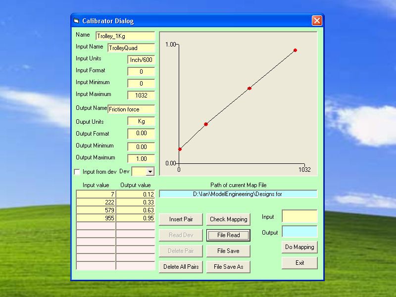
The only spring balance I could find in local shops was for measuring weights up to 10 Kilograms. A few calculations show that a 10 Kilogram frictional force on the rim of a 10 cm wheel is going to dissipate about 30 joules per revolution which, at a speed of 1200 rpm (=20rps) corresponds to a power of 600 watts which is a lot of power for a small engine. And so I decided to replace the spring balance with a precision spring chosen from a set according to the range of power to be measured, and to measure the position of the trolley on which the wooden block is mounted with a linear optical encoder (US Digital EM1 Encoder Module 150 lines/inch), the graduated tape of which is fixed underneath the trolley. Arduino acquires the Quadrature output which reveals motion of the tape through the encoder. A Quadrature signal consists of two digital square waves with a phase difference of +90 or -90 depending on the direction of the motion. The Arduino reveals the transitions on these two signals and maintains an integration counter, which represents the position of the trolley in units of 1/600 inch. The trolley has an excursion of 44mm so the maximum value of the counter is about 1040. Test Bench software on the PC then uses table interpolation to recover the corresponding frictional force in Kilograms. The values in the table, which depend on the spring being used, are defined by a Calibration Process about which more later.
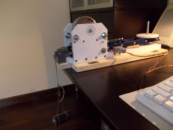
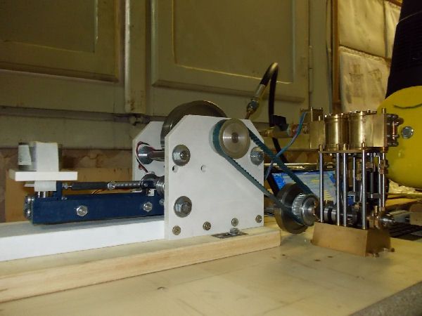
The picture below shows the Arduino with the connecting cable to the instrument.

P1-02Arduino_zpsc0143bba.jpg


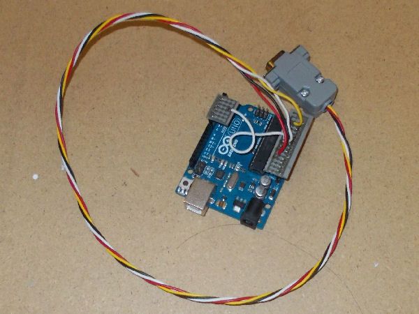
This cable has five wires:
  • 0V (black)
  • +5V (red)
  • Square wave from infrared fork sensor for wheel revolutions (white)
  • Square wave A from linear encoder for trolley position (orange)
  • Square wave B from linear encoder for trolley position (yellow)
My next post will describe the hardware of the instrument itself.
 
[SIZE=+2]AN INSTRUMENT FOR MEASURING THE POWER DELIVERED BY SMALL ENGINES[/SIZE]

THE INSTRUMENT HARDWARE


The instrument is composed of a wooden base and four main assemblies:
  • Rocker Assembly and Springs
  • Trolley Assembly
  • Wheel Assembly and Base
  • Calibration Accessory
Rocker Assembly and Springs

P2-02RockerParts_zpsf4644cd6.jpg

P2-02RockerAssy_zps03ba67c3.jpg

P2-03RockerEncoderCloseup_zpsbb975adc.jpg


This first version of the Rocker shown in the above pictures is built from two steel rails held together by steel cross ribs. The linear encoder sensor is mounted on an aluminum angle bracket at the right of the assembly. Between this bracket and the second cross rib is the pivot axle on which the Rocker rocks. The excursion of the trolley along the rails is limited by two stops, one at the extreme right and one to the left of the axle. Between the third and fourth cross ribs is the fixed hook for the spring.

The white disk on the left is a platform for weights to adjust the pressure of the wooden block against the rim of the wheel.

The Rocker Assembly includes the cable which connects the two sensors to the connector which is mounted on the Base with an aluminum support. The wires to the trolley position sensor (i.e. the linear encoder) pass through a hole in the rear rail. This sensor can be seen with the slot in which the graduated tape passes without touching.

P2-04RockerShortInUse_zpsdc213c44.jpg

P2-05RockerShortBit_zpsc8a495a0.jpg


Initial runs revealed that, even with no weights on the platform, this Rocker caused two much pressure on the wooden block. The solution was to cut it in half and provide a simple plug-in mechanism to allow the two halves to be joined together when required; in addition a small platform for weights can be plugged into the top of the spring support . The two pictures above show this modification.

P2-06SetOfSprings_zps28329cb3.jpg


This last picture shows the set of four alternative springs, each with an appropriate arm so that they all have the same overall length. They have a maximum tension of 1Kg, 2Kg, 3Kg and 4Kg respectively. Note that all the springs require a certain minimum load before starting to expand.

Trolley Assembly

P2-07TrolleyParts_zps645876e1.jpg

P2-08TrolleyAssyTop_zpse110fa1b.jpg

P2-09TrolleyAssyBottom_zps2d25ef96.jpg


The hook on the left is for linking to the business end of the spring. The hook on the right is used together with the Calibration Accessory during the Calibration Process.

The third picture shows the underside of the trolley with the arrangement for holding the graduated mylar tape of the linear encoder. The four brass pins are legs which allow the trolley to be placed on a flat surface without damaging the rather delicate tape.

P2-10TrolleyOnRocker_zpsea4cd638.jpg


This last picture shows the Trolley mounted on the Rocker. In this position the graduated Mylar tape slips through the slot in the Encoder without touching the sides or the bottom.

Wheel Assembly and Base

P2-11WheelParts_zps30cb57c0.jpg

P2-12WheelAssy_zpsb295c30d.jpg


The two side supports are made from 1cm thick white PVC plate. Two ball bearings support the 12mm diameter axle which is in steel. The wheel is in steel and has a diameter a shade under 100mm. The disc with the cutout to alternately block and pass the infrared beam is made from PVC. I had to paint the disc itself black because enough beam was shining through the translucent white plastic to trigger the sensor. The toothed pulley receives the rotational energy from the engine under test.

P2-13WheelAssyOnBase_zps6fa2f47b.jpg


This last image shows the Wheel Assembly mounted on its Base. Note the four slots in the lower piece of the Base which allows the instrument to be moved horizontally about 15mm to facilitate setting the appropriate tension in the toothed belt.

Calibrator Accessory

P2-14CalibratorParts_zps243deb5f.jpg

P2-15CalibratorAssy_zps159d5d5c.jpg


The Calibrator Accessory is used during the Calibration Process to help apply a series of known horizontal forces to the Trolley in order to define the values in the interpolation table used by the Test Bench software to map the trolley position signal from the linear encoder under the trolley to force units. It’s use is covered in a later section.

P2-16CalibrationWeights_zps32e835cb.jpg


This last picture shows some of the assortment of ad-hoc weights I used during calibration of the four springs.

Complete Instrument

P2-17InstrumentBack_zpsb48e62b3.jpg

P2-18InstrumentFront_zps80e91ca2.jpg

P2-19InstrumentGuts_zps2d46742d.jpg


These pics show the assembled power meter with the smallest of the springs (1Kg) mounted in place.

P2-20InstrumentWithEngine_zpsebf2a116.jpg


This image shows the instrument and the smallest of my steam engines mounted on a big wooden platform and connected via the toothed belt between the identical toothed pulleys, one of the shaft of the motor and one on the shaft of the instrument’s brake wheel. The other fixing holes visible in the platform are for other engines.

My next post will describe the Pressure Sensor and the Test Bench (ie the software of the instrument).
 
[SIZE=+2]AN INSTRUMENT FOR MEASURING THE POWER DELIVERED BY SMALL ENGINES[/SIZE]

THE PRESSURE SENSOR

Following advice received from several HMEM members I ordered a Honeywell TruStability series sensor from Mouser. These are piezo-resistive silicon pressure sensors with integrated electronics to provide temperature compensation and the capacity to communicate the output pressure values as 14 bit digital integers. The particular sensor I bought reads pressures from 0 up to 10 bar relative to the ambient pressure and delivers the output via the well known I2C bus which is directly supported by Arduino. Here is a picture of the sensor itself (taken from the Honeywell Product Brief). The pressure to be measured must be supplied at the barbed tube of the sensor. The overall height of the sensor is a bit less than 20mm.

P3-01PressureSensor_zpsc65792ac.jpg


To allow the sensor to be inserted easily between the compressed air line and the input of the engine under test, I built a brass housing as shown in the following two pictures. Two wires are for 0V and +5V and two are for the I2C bus.

P3-02PressureSensorInCase_zps0b33bbb1.jpg
.
P3-03PressureSensorWithLidOff_zps6903ef08.jpg


THE TEST BENCH

This section gives a brief description of the Test Bench software I developed last summer while away from home. As implied by the name, I made it more general and capable than was necessary for simply measuring engine power.

Overview

The Test Bench is a software tool for use with a PC connected via a USB cable to a front end Arduino micro-computer. In normal use, various devices (sensors and perhaps also actuators) of some Physical System under test would be connected to the IO pins of the Arduino.
The aim of the Test Bench is to provide a software framework to simplify and hence speed up the process of measurement of aspects of the Physical System under test. The Test Bench software contains a relatively small component which is loaded into Arduino and which enables it to adapt to and drive a device configuration which it receives as data from the PC. During a test run, the information to the actuators and from the sensors of the current configuration flows between Arduino and PC via the USB cable.

The Test Bench software component for the PC is more complex but follows the same philosophy namely to express the ability to handle types of device and, in addition, types of Meter, but to receive the definition of the actual configuration of Devices and Meters as data held in Configuration files. A Meter has it’s driver on the PC and has the ability to manage one or more devices. An example is a PID controller which can manage the value output by an actuator device to maintain at some predefined set point the value of a sensor device connected via an ADC, an Encoder or some I2C sensor.


So far I have implemented the following Device Types:
  • Square wave generator
  • Pulse sensor
  • Analogue input sensor
  • PWM ( Pulse Width Modulation) output generator
  • Quadrature encoding generator
  • Quadrature encoding Sensor
  • Stepper Motor Driver
  • I2C input sensor
and the following Meter types:
  • Brake Power meter
  • PWM Wave meter
  • Revs Injector meter
  • PID Controller
Defining a Configuration

To use the Test Bench for a certain task, the first step is to define the Configuration in terms of Devices and Meters. For the measurement the power of a steam engine running under compressed air the Configuration has three Devices and one Meter. The Devices are
  • a Pulse Sensor for acquiring the wheel revs,
  • a Quadrature Sensor for acquiring the position of the Trolley and converting this position to a frictional force in kilograms,
  • an I2C Input Sensor for acquiring the signal from the pressure sensor in the air supply and converting it to a pressure in bar.
The Meter in the configuration is a Brake Power meter which has as parameters:
  • the diameter of the friction wheel
  • engine geometry (cylinder diameter, stroke, number of power strokes per rev)
and which uses the values acquired by the three Meters to compute the instantaneous Brake Power, the power absorbed from the air supply, and the Efficiency.

P3-04TB_ConfigurationDialog_zps88e60493.jpg


The picture above shows the Test Bench dialog for defining this Configuration and saving the definition in a text file. Note that the declarations for the Quadrature Sensor and the Pressure Sensor include the names of the text files containing the respective Calibrator tables for mapping the value acquired by the sensor to the required physical units (ie Kilograms and Bar respectively) Note too that the declaration of the Meter nominates the Devices from which it must get its data to perform the calculations.

Scenarios


The information in a configuration file does not define all the information needed to start a particular test run. The missing information includes:
  • which Devices and Meters are to be enabled
  • values for the parameters of Devices and meters
  • the sampling period
  • whether logging is enabled or not
  • the directory in which to save the log file
  • a short descriptive note for the run
All this information can be inserted manually on the main dialog described below. Once this has been done it can be saved in a Scenario file for reuse.

Running tests and recording results

Once a Configuration has been defined it can be loaded into the Test Bench as the current configuration. If available, a Scenario can be loaded to prepare for a test run.

P3-05TB_MainDialog_zps35140575.jpg


The above picture shows the Test Bench main dialog after the configuration defined above and an appropriate Scenario have been loaded. Across the top of the dialog is the main menu. Four frames summarize the current state of the three Devices and the Meter. Note that the participation in a particular Test Run of Devices and Meters can be individually enabled or disabled. Output values are shown both as numbers and as a cursor along a linear scale.

Down the right edge of the dialog is a Control Frame used principally to set the sampling frequency and to start and stop test runs. It also shows the utilizations of the Arduino CPU and USB based bi-directional messaging link with the PC, and .supports read and write operations to a specified Arduino pin.

To start a run one clicks on the Start button in the Control Frame. During the Run the values output by the Devices and Meters are updated on the screen at the sampling frequency. If logging is enabled then the values of parameters and outputs of the devices and meters is recorded in memory at the sampling frequency during the test run. If desired the values of Device and Meter parameters can be modified on the fly i.e. while a run is in progress.

The run can be terminated at any time by clicking the Stop button on the Control Frame. If logging was enabled then the collected log data for the run is written to a log file on disk.

Examining result logs

Once the necessary run results have been collected in the form of log files in a common directory, the Test bench supports a simple but useful facility to selectively examine the data. Upon activation from the Log menu, the Test Bench collects the data from all the log files into a single relational data base and then allows the user to select which data to show in tabular and graphic form. The selection can relate to a combination of logs and two or three, names of parameters and/or outputs. In addition the user may specify a logical criteria which the selected data must satisfy (using the rules of an SQL where clause) and must specify which of the chosen parameter or outputs must be used as the abscissa on the graph.

P3-06LogDataDialog_zps1e21486f.jpg

P3-07LogDataGraph_zpsb91ed3e3.jpg


The above pictures show the dialog used for examining the data and a closeup of an example of the graphic representation. This example shows the input pressure and the wheel revs (WR_PulseRate) as ordinates with the elapsed run time in seconds on the abscissa taken from the log of one of the runs to measure the performance of an engine. Note that at the start of the run, both the pressure and the revs take some time to reach the start of the regular smooth descent.

Frictional Force Sensor Calibration Process

The pictures below show the instrument setup for the calibration process. The fruit of the calibration process is an interpolation table for mapping the linear encoder counter values into a force in Kilograms.

P3-08CalibrationSetup1_zps161cb56d.jpg

P3-09CalibrationSetup2_zpsc2c106d7.jpg


The Calibrator Accessory can be seen with its pulley bearing the cord via which the suspended weight exerts a horizontal force on the trolley. The instrument is connected via Arduino to the PC on which the Calibration Dialog of the Test Bench is running. Below is a screen snap of this dialog.
P3-10CalibrationDialog_zps4e2a9127.jpg

Each row of the mapping table is defined by inserting the Output Value from the keyboard and acquiring the Input Value by pressing the Read Dev button which causes the Test Bench to tell Arduino to read the input value of the selected device driver (which must be enabled), and send this digital number back to the Test Bench for insertion in the mapping table.

My next post will describe the first attempt to use the instrument to measure the performance of an engine.
 
Last edited:
[SIZE=+2]AN INSTRUMENT FOR MEASURING THE POWER DELIVERED BY SMALL ENGINES[/SIZE]

FIRST USE EXPERIENCE

Set up and Approach

For the first serious attempt to measure the performance of an engine I chose the two cylinder engine I completed a year ago, the [thread=20023]build log[/thread] of which is on this forum.

P4-01TestSetupDiagram_zps32a18be9.jpg


The diagram above illustrates the complete setup for testing this engine.

P4-02TestSetupEngInstru_zpsf2fa633c.jpg

P4-03TestSetupEngPsensArd_zpseae5f428.jpg

P4-04TestSetupPcArdEng_zpsb7954178.jpg


The three pictures above show the setup for testing this engine. All the components were arranged on the workshop bench. During the eight runs, both the short and long configurations of the Rocker were used.

The air pressure is supplied by a simple (and very noisy!) 25 liter compressor with a tap at the outlet but with no ability to maintain a constant pressure under load. On the Brake Power Instrument itself, the frictional force between the wooden block and the wheel can be regulated by placing more or less weight on the platform at the end of the rocker, but there is no mechanism for regulating this weight in real time to maintain a constant frictional force.

A pressure sensor measures the air pressure P at the input to the engine. The instrument itself measures the revolution rate R of the engine and the frictional resistance F of the wooden block against the wheel of the meter. Test Bench software on the Arduino receives these three values and, at the sampling frequency, communicates them via the USB cable to the Test Bench software on the PC. On the PC, the a Meter computes the instantaneous absorbed power and the instantaneous delivered brake power and the efficiency. Again at the sampling frequency all the potentially useful data is memorized, and at the end of each run, this data is written to a log file on disk.


Since there is no means of keeping any single one of these three variables constant during a test run I accept that all three are going to change. For simplicity I decided that, for a given engine, the test will consist of a number of runs in which:
  • the initial air pressure will have the same value for all runs
  • the compressor motor will be off during a run (and hence the pressure will fall continuously during a run)
  • the weight on the rocker platform will be constant during any given run but will be progressively increased from run to run.
Each of these runs will yield a log file from which four quantities can be extracted as continuous functions of the elapsed run time t (which the Test Bench calls the Period Time) namely:
  • the Pressure P(t) in bars
  • the Revs R(t)
  • the delivered Power P(t) in watts
  • the Efficiency E(t) as a percentage
A preliminary inspection of their graphs showed that, ignoring the initial seconds during which the engine is accelerating and the conditions are settling down, these functions are all very smooth apart from a certain jitter between adjacent samples. Each could therefore be well approximated by a suitable quadratic function of t. The three coefficients of each quadratic could be determined by using a reliable curve-fitting algorithm which I had already taken from a very useful book bought years ago called Numerical Recipes in Fortran.

At that point, for each of chosen number of fixed values for the Pressure P, I could recover from each log the corresponding values for Revs, Power and Efficiency. Simply solve the Pressure quadratic for the Period Time t and then insert that value of t into the quadratics for Revs, Power and Efficiency. Then if there are N log files, for each of these constant pressure values I will have N points for each of two curves showing how Power and Efficiency vary with Revs.

Doing it


To implement this data processing I wrote a custom program which takes as input the database prepared by the Test Bench log analysis feature and which generates the output data as CSV (Comma Separated Values) text files for use by the graph drawing capabilities of Excel. These outputs are:
  • a CSV file for each log showing the data point and the fitted curve values for each of the four functions
  • a CSV file with the Revs, Power and Efficiency values for each of the constant pressure values.
P4-05AdhocProgramDialog_zpsa47bc374.jpg


The above picture shows the launch dialog of this custom program. The inputs are the path of the data base file, the range and step for the constant pressure values and, for each log, optional values for the minimum and maximum of the Period Time to be used. The dialog is shown after all these inputs have been inserted.

P4-06FittedCurvesShort616gms_zpsdd98c20a.jpg


This picture shows the Excel graphs for the data and fitted curve values for each of the four functions extracted from one of the eight log files. Note that the jitter in the data is greater at the beginning of the run, when the pressure, and hence the revs, are higher. In all four cases the fitted curve appears to provide a very good approximation to the data points from which it is derived.

P4-07V2PerformanceCurves_zps26dc6fd8.jpg


This picture shows the Excel graphs for the constant pressure performance curves for Power and Efficiency as functions of Revs. Each curve has eight data points, one derived from each of the eight log files. Some evidence of the peak I expected occurs only for the Efficiency curve at the lowest constant pressure (1.5 bar). Otherwise, for any given input pressure, both the output power and the efficiency decrease as the revolutions increase. This must be due to the steady increase with revs (probably worse than linear) of power dissipation in the engine itself.

Coefficient of Friction

A final remark relates to the Coefficient of Friction between the rim of the steel wheel and the wooden block. It was because I had no idea of the value of this coefficient that I discovered only after the first attempts to use the instrument that the rocker was too long and heavy to create a light load for an engine, and so I had to cut it in two to have a short version when necessary.

The log results of the test runs reported above allowed me to produce an estimate of this coefficient. The values varied a little from run to run and also during each run but the values are centered around 0.3. Thus a radial force of 1 Kg between the wooden block and the wheel rim generates a tangential frictional force on the wheel of roughly 0.3 Kg.
 
I have a table somewhere that shows coefficient of friction values for some materials. But this looks interesting.
 
.

A lot of machining and heavy and clunky Victorian design mechanical hardware needed there.

Wouldn't it be a lot easier to have a water pump connected to the engine and measure the flow rate in a re-circulating water system ?
Gradually increasing the water volume or the water pumped height until the engine cannot pump at any higher flow rate any more.

.
 
Hello Dave,

As a matter of fact I did consider pumping some fluid against gravity as a way of providing a measurable load for small engines. In the end I plumped for the Seller Dynamometer technique for three reasons.
  • The fact that Seller’s idea gets enthusiastic recommendation in Harris’s book gave me some confidence that the method would probably work in practice. Harris doesn’t mention pumping fluid as an alternative.
  • Personally I know very little about hydraulics and pumps and would have had difficulty in choosing or building the pump and the flow sensor or in estimating losses due to turbulence.
  • Rough calculation, ignoring losses due to turbulence and friction in the pump, show that rather a lot of fluid would be involved. For example, if I’ve got my sums right, a 100 watt motor would pump over 10 litres of water per second up 1 meter against gravity. Or 5 litres per second up 2 meters, but a 2 meter height is rather awkward to organise in my little workshop which is exactly 2 meters high.. Which has implications for the size and cost of the pump and the flow sensor. A popular 10 dollar flow sensor I’ve seen on the Arduino forum has inlets and outlets with ½” tubes but has a maximum flow rate of only ½ litre per second.
So to answer your question “would it be a lot easier..?” I have to answer that I don’t think it would have been easier for me. Not even bearing in mind that building my brake power meter certainly wasn’t as easy as I thought it would be when I started! But the only way to know the answer would be to try to do it.
 
Back
Top